Pricing Binary Options
By Aman Jindal, CFA, FRM, CQF
The following code uses Monte Carlo Simulations to price Binary Options.
Option Valuation Formula:
The fair value of an option is the present value of the expected payoff at expiry under a risk-neutral random walk for the underlying.The risk-neutral random walk for the underlying S is: $$ ds = rS dt + \sigma SdX $$
This is simply our usual lognormal random walk but with the risk-free rate instead of the real growth rate.Thus,
$$ optionValue = e^{-r(T-t)}E^Q[Payoff(S_T)] $$For Binary Call Option: Payoff = 1 if $S_T>K$ ; 0 otherwise
For Binary Put Option: Payoff = 1 if $S_T<K$ ; 0 otherwise
Algorithm Used:
- Simulate the risk-neutral random walk starting at today’s value of the asset $S_0$ over the required time horizon. This gives one realization of the underlying price path.
- For this realization calculate the option payoff.
- Perform many more such realizations over the time horizon.
- Calculate the average payoff over all realizations.
- Take the present value of this average, this is the option value.
Euler-Maruyama Method of simulating the stock Price:
To apply Euler-Maruyama method, we first divide the interval T into M intervals such that $ \delta t = \frac {T}{M}$
Then, stock price (S) is simulated as
$$ \delta S = rS\delta t + \sigma S \sqrt {\delta t} \phi$$where $\phi$ is from a standard Normal distribution
Errors:
Let $\epsilon$ be the desired accuracy in our Monte Carlo Simulation(MCS). Errors in MCS will arise due to:
- $O(\delta t)$ due to Size of the time step $\delta t$
- $O(N^{-0.5})$ due to N finite number of simulations
Thus, for chosen levels of $\epsilon$ we can choose:
- $O(\delta t) = O(\epsilon)$ and thus, number of time steps, $M = \frac{1}{\delta t}$
- Number of simulations, $N=O(\epsilon ^{-2})$
Inputs chosen for the Analysis:
- The error levels chosen are [0.2,0.1,0.05,0.02,0.01]
- Thus, number of time steps(M) are [5,10,20,50,100]
- Thus, number of simulations(N) are [25,100,400,2500,10000]
Plotting Option Prices against Stock Prices:
- Stock Prices have been varied from 1 to 200 in a step of 1
- Four different Time to Expiry have been chosen [0.25,0.5,1.5,2]
- Four different Volatility have been chosen [0.1,0.15,0.25,0.3]
- Four different Risk-Free rate have been chosen [0.03,0.04,0.06,0.07]
- The default values are S = 100, K = 100, T = 1,r = 0.05, $\sigma = 0.2$, M = 50, N = 2500
Plotting Option Prices against Volatility, Risk-Free Rate and Time to Maturity:
- Three StockPrice = [90,100,110] for simulating OTM,ATM,ITM options have been taken
- Volatility has been varied in the interval (0.01,0.6)
- Risk-Free Rate has been varied in the interval (0.01,0.2)
- Time to Maturity has been varied in the interval (0.1,2)
# Importing Libraries

import math
import numpy as np
import numpy.random as npr
import pandas as pd
import matplotlib.pyplot as plt
from scipy.stats import norm
plt.style.use('seaborn')
# Creating a Folder, if none exists, within cwd to store the Images

images_folder = 'Images'   # Folder Name within the cwd where Images will stored
cwd = os.getcwd()
images_folder_path = os.path.join(cwd, images_folder)

if not os.path.exists(images_folder_path):
    os.makedirs(images_folder_path)
# Function for Valuation by BSM

def BSValue(S,K,T,r,vol,optionType):
    d2 = (np.log(S/K) + (r - 0.5*vol**2) * T) / vol / np.sqrt(T)
    if optionType == 'Call':
        optionPrice = np.exp(-r * T)*norm.cdf(d2)
    elif optionType == 'Put':
        optionPrice = np.exp(-r * T)*norm.cdf(-d2)
    else:
        optionPrice = np.nan
    return optionPrice
# Function for Valuation by Monte Carlo Simulations

def MCValue(S0,K,T,r,vol,optionType,M,N):
    S = np.full(N,S0,dtype=np.double)
    dt = T/M
    for i in range(M):
        S = S*(1 + r*dt + vol*np.sqrt(dt)*npr.randn(N)) # Euler-Maruyama Method
    if optionType == 'Call':
        optionPrice = np.exp(-r*T)*np.mean(np.where(S>K,1,0))
    elif optionType == 'Put':
        optionPrice = np.exp(-r*T)*np.mean(np.where(S<K,1,0))
    else:
        optionPrice = np.nan
    return optionPrice
# Defining Parameters

sDefault = 100
kDefault = 100
tDefault = 1
rDefault = 0.05
volDefault = 0.2
mDefault = 50     # Number of Time Steps
nDefault = 2500   # Number of Simulations

S = np.arange(1,201,1,dtype='float')
T = [0.25,0.5,1.5,2]
r = [0.03,0.04,0.06,0.07]
vol = [0.1,0.15,0.25,0.3]
error = [0.2,0.1,0.02,0.01]
# Calculation Number of Steps and Simulations

M = []
N = []
for i in error:
    M.append(int(round(pow(i,-1))))
    N.append(int(round(pow(i,-2))))
print("M = {}".format(M))
print("N = {}".format(N))
# Option Prices for different Stock Prices (S) and number of Simulations (N)

stockPrices = S.size
simulationCounts = len(N)

BSCall = np.zeros((stockPrices,1))
BSPut = np.zeros((stockPrices,1))
MCCall = np.zeros((stockPrices,simulationCounts))
MCPut = np.zeros((stockPrices,simulationCounts))

for i,s in np.ndenumerate(S):

    BSCall[i,0] = BSValue(s,kDefault,tDefault,rDefault,volDefault,'Call')
    BSPut[i,0] = BSValue(s,kDefault,tDefault,rDefault,volDefault,'Put')

    for j,(m,n) in enumerate(zip(M,N)):

        MCCall[i,j] = MCValue(s,kDefault,tDefault,rDefault,volDefault,'Call',m,n)
        MCPut[i,j] = MCValue(s,kDefault,tDefault,rDefault,volDefault,'Put',m,n)
print('Calculations Done')
# Plotting Results of MCS for Binary Call for different S and N

image_name = 'image1.png'       # Name of the Image File
image_path = os.path.join(images_folder_path, image_name)

fig, ((ax1,ax2),(ax3,ax4)) = plt.subplots(2,2,sharex = True, sharey = True)
axs = [ax1,ax2,ax3,ax4]
for i,ax in enumerate(axs):

    ax.plot(S,BSCall[:,0], label='BSM')
    ax.plot(S,MCCall[:,i], label='MCS: N = {}'.format(N[i]))
    ax.set_ylim(-0.05,1.05)
    ax.tick_params(labelsize=9)
    ax.legend(fontsize=8,frameon=True)

fig.text(0.5, 0.04, 'Stock Price', ha='center')
fig.text(0.04, 0.5, 'Binary Call Price', va='center', rotation='vertical')
fig.suptitle("Binary Call Price with varying number of simulations",ha='center')
fig.tight_layout()
fig.subplots_adjust(left = 0.14,top=0.92, bottom = 0.14);

plt.savefig(image_path, dpi=300)
plt.close();
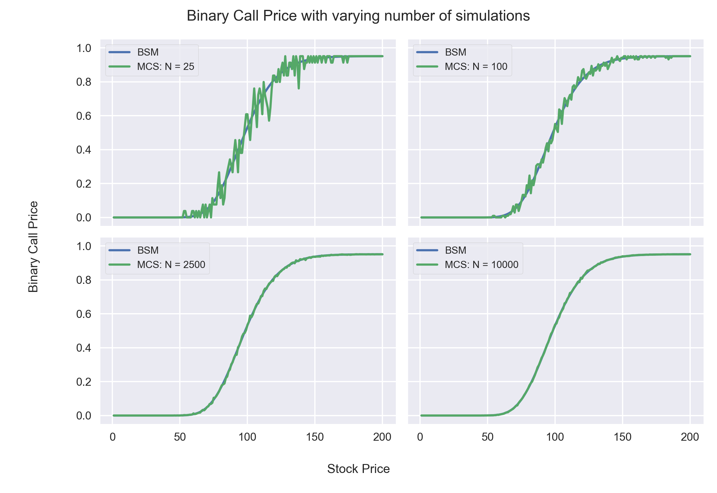
Observations:
- We can infer from the above graphs that as the number of simulations increase, the results of Monte Carlo Simulations get closer to the theoretical value obtained from the Black Scholes Merton Model.
- The slope of the graph is highest for ATM (At the Money) Option.
The following table provides a snapshot of the Binary Call Prices for S in the interval [95,105]
df = pd.DataFrame(data=BSCall,index=S,columns=['BSM'])
df1 = pd.DataFrame(data=MCCall,index=S,columns=['MCS: N=25','MCS: N=100','MCS: N=2500','MCS: N=10000'])
df = df.join(df1)
df.index.rename('Stock Price',inplace=True)
print ("\033[1m\t\t\033[4mBinary Call Option Valuation\033[0m\033[0m")
df.loc[95:105]
# Plotting Results of MCS for Binary Put for different S and N

image_name = 'image2.png'       # Name of the Image File
image_path = os.path.join(images_folder_path, image_name)

fig, ((ax1,ax2),(ax3,ax4)) = plt.subplots(2,2,sharex = True, sharey = True)
axs = [ax1,ax2,ax3,ax4]
for i,ax in enumerate(axs):

    ax.plot(S,BSPut[:,0], label='BSM')
    ax.plot(S,MCPut[:,i], label='MCS: N = {}'.format(N[i]))
    ax.set_ylim(-0.05,1.05)
    ax.tick_params(labelsize=9)
    ax.legend(fontsize=8,frameon=True)

fig.text(0.5, 0.04, 'Stock Price', ha='center')
fig.text(0.04, 0.5, 'Binary Put Price', va='center', rotation='vertical')
fig.suptitle("Binary Put Price with varying number of simulations",ha='center')
fig.subplots_adjust(left = 0.14,top=0.92, bottom = 0.14);

plt.savefig(image_path, dpi=300)
plt.close();
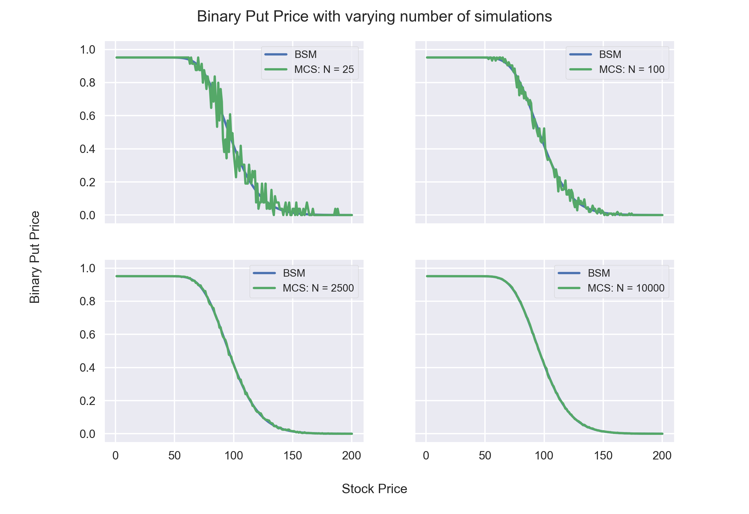
Observations:
- We can infer from the above graphs that as the number of simulations increase, the results of Monte Carlo Simulations get closer to the theoretical value obtained from the Black Scholes Merton Model.
- The magnitude of slope (Delta) of the graph is highest for ATM (At the Money) Option.
The following table provides a snapshot of the Binary Put Prices for S in the interval [95,105]
df = pd.DataFrame(data=BSPut,index=S,columns=['BSM'])
df1 = pd.DataFrame(data=MCPut,index=S,columns=['MCS: N=25','MCS: N=100','MCS: N=2500','MCS: N=10000'])
df = df.join(df1)
df.index.rename('Stock Price',inplace=True)
print ("\033[1m\t\t\033[4mBinary Put Option Valuation\033[0m\033[0m")
df.loc[95:105]
# Calculating Errors for different S and N

temp = np.hstack((BSCall,BSCall,BSCall,BSCall))
temp1 = np.hstack((BSPut,BSPut,BSPut,BSPut))

errorCall = temp - MCCall
errorPut = temp1 - MCPut
print('Calculations Done')
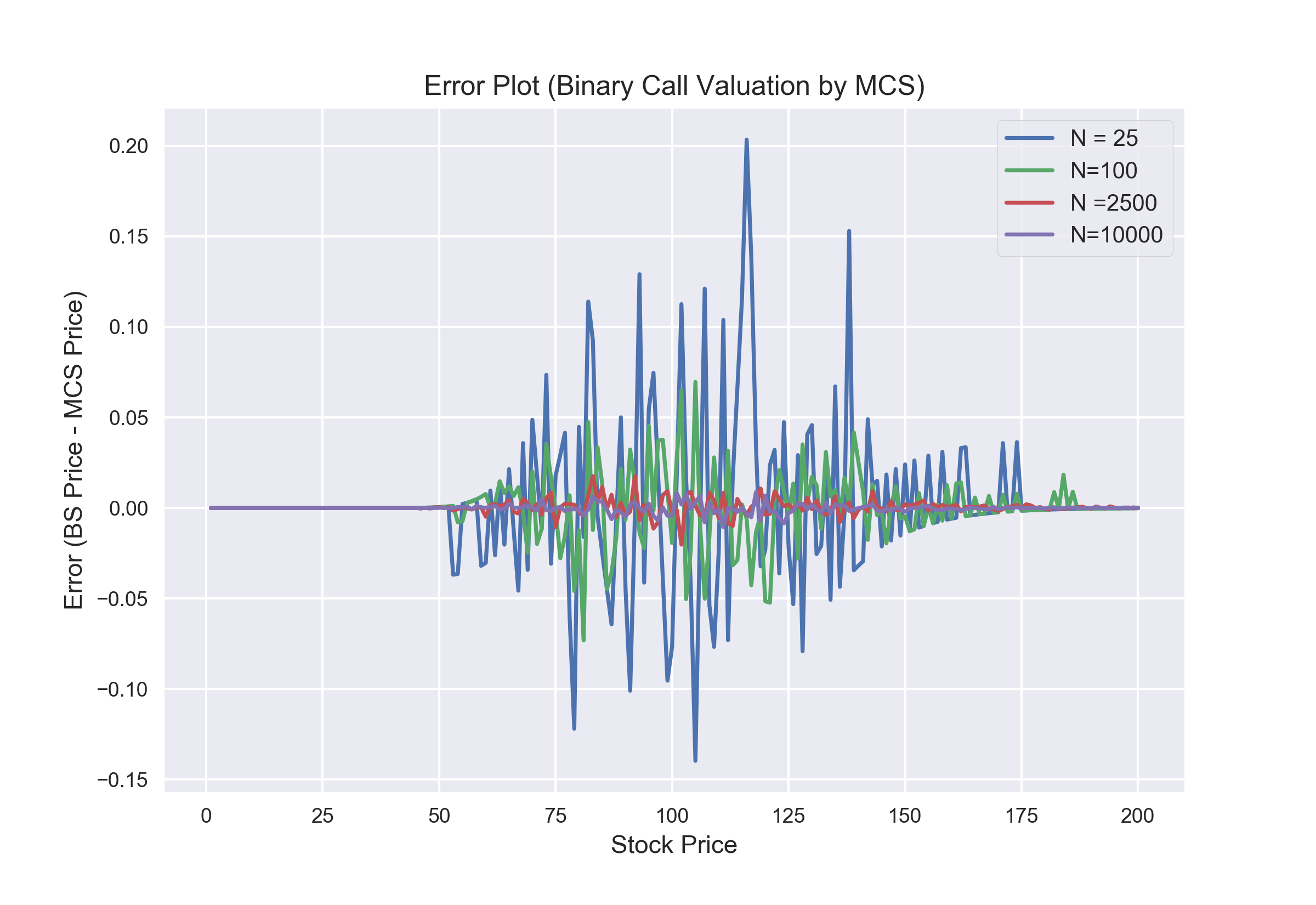
# Plotting Errors in Binary Call Valuation for different S and N

image_name = 'image3.png'       # Name of the Image File
image_path = os.path.join(images_folder_path, image_name)

plt.figure()
plt.plot(S,errorCall)
plt.legend(['N = 25', 'N=100','N =2500','N=10000'],frameon=True)
plt.xlabel('Stock Price')
plt.ylabel('Error (BS Price - MCS Price)')
plt.xticks(fontsize=9)
plt.yticks(fontsize=9)
plt.title('Error Plot (Binary Call Valuation by MCS)');
plt.savefig(image_path, dpi=300)
plt.close();
# Plotting Errors in Binary Put Valuation for different S and N

image_name = 'image4.png'       # Name of the Image File
image_path = os.path.join(images_folder_path, image_name)
plt.figure()
plt.plot(S,errorPut)
plt.legend(['N = 25', 'N=100','N =2500','N=10000'],frameon=True)
plt.xlabel('Stock Price')
plt.ylabel('Error (BS Price - MCS Price)')
plt.xticks(fontsize=9)
plt.yticks(fontsize=9)
plt.title('Error Plot (Binary Put Valuation by MCS)');
plt.savefig(image_path, dpi=300)
plt.close();
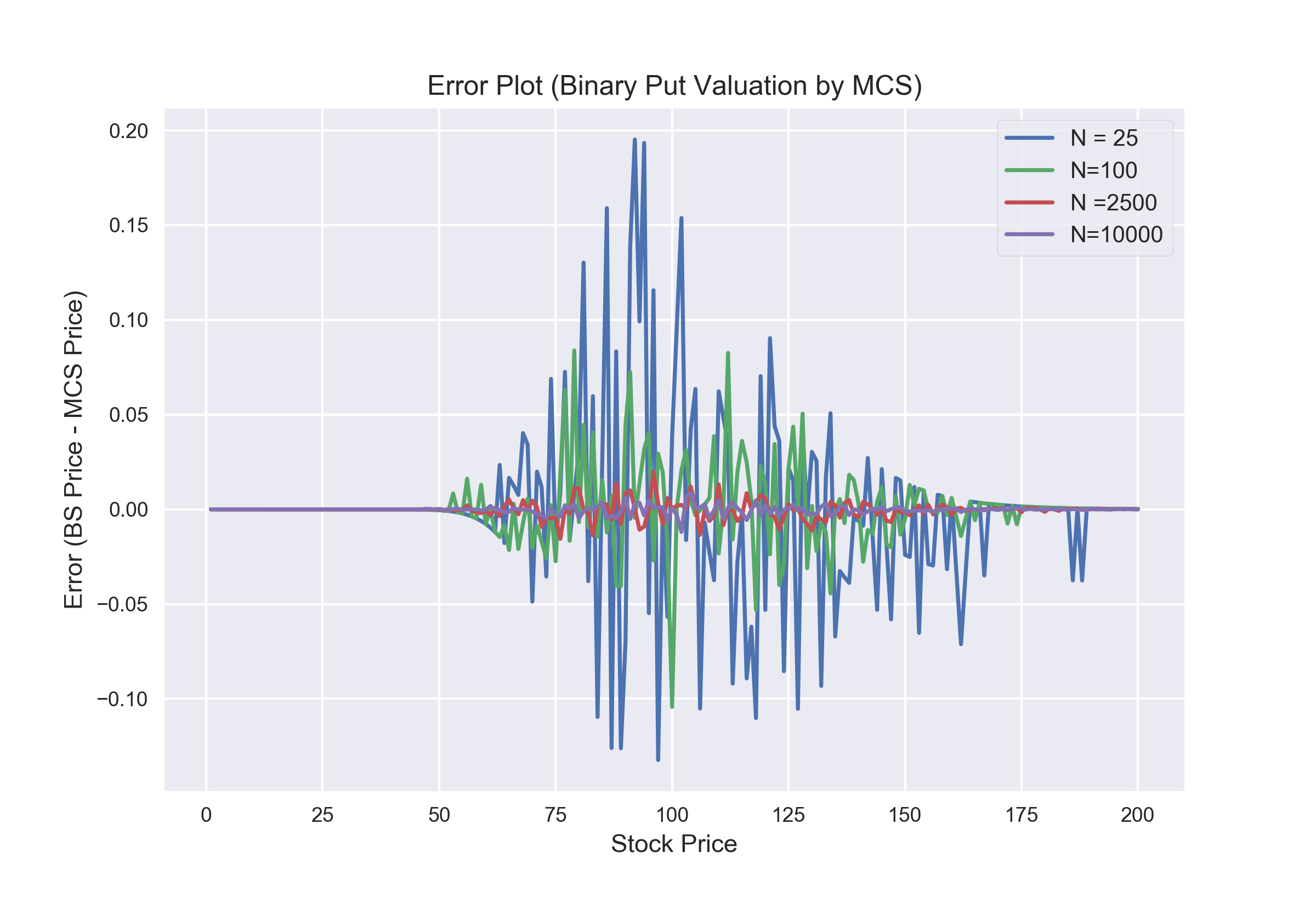
Observations:
- From the above two graphs we can infer that as the number of simulations and the number of Time steps increase, the results form the Monte Carlo Simulations get closer to the theoretical values from the BSM Model.
- Errors are larger when Stock Price (S) is closer to Strike Price (K).
# Option Prices for different Stock Prices (S) and volatility (Vol)

stockPrices = S.size
volCount = len(vol)

BSCallVol = np.zeros((stockPrices,volCount))
BSPutVol = np.zeros((stockPrices,volCount))
MCCallVol = np.zeros((stockPrices,volCount))
MCPutVol = np.zeros((stockPrices,volCount))

for j,sigma in enumerate(vol):
    for i,s in np.ndenumerate(S):
        BSCallVol[i,j] = BSValue(s,kDefault,tDefault,rDefault,sigma,'Call')
        BSPutVol[i,j] = BSValue(s,kDefault,tDefault,rDefault,sigma,'Put')
        MCCallVol[i,j] = MCValue(s,kDefault,tDefault,rDefault,sigma,'Call',mDefault,nDefault)
        MCPutVol[i,j] = MCValue(s,kDefault,tDefault,rDefault,sigma,'Put',mDefault,nDefault)
print('Calculations Done')
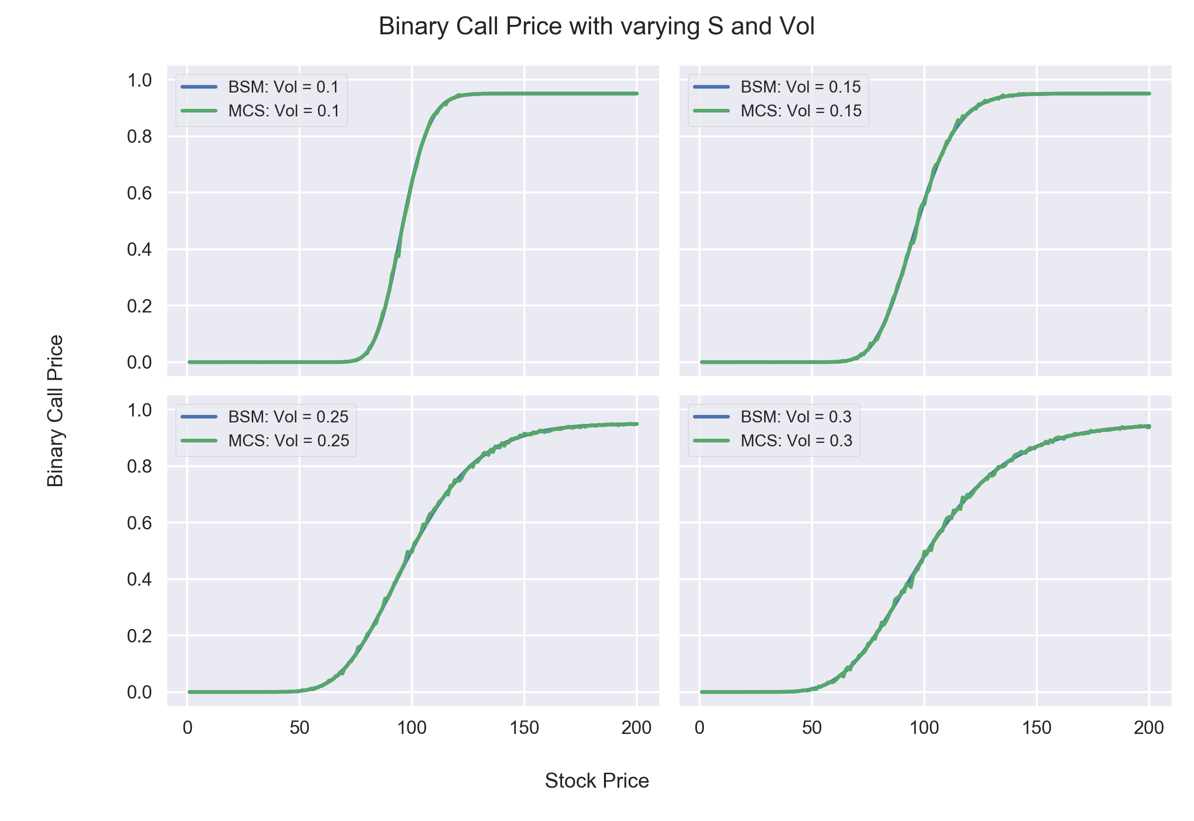
# Plotting Results of MCS for Binary Call for different S and Vol

image_name = 'image5.png'       # Name of the Image File
image_path = os.path.join(images_folder_path, image_name)
fig, ((ax1,ax2),(ax3,ax4)) = plt.subplots(2,2,sharex = True, sharey = True)
axs = [ax1,ax2,ax3,ax4]
for i,ax in enumerate(axs):

    ax.plot(S,BSCallVol[:,i], label='BSM: Vol = {}'.format(vol[i]))
    ax.plot(S,MCCallVol[:,i], label='MCS: Vol = {}'.format(vol[i]))
    ax.set_ylim(-0.05,1.05)
    ax.tick_params(labelsize=9)
    ax.legend(fontsize=8,frameon=True)

fig.text(0.5, 0.04, 'Stock Price', ha='center')
fig.text(0.04, 0.5, 'Binary Call Price', va='center', rotation='vertical')
fig.suptitle("Binary Call Price with varying S and Vol",ha='center')
fig.tight_layout()
fig.subplots_adjust(left = 0.14,top=0.92, bottom = 0.14);
plt.savefig(image_path, dpi=300)
plt.close();
# Plotting Results of MCS for Binary Put for different S and Vol

image_name = 'image6.png'       # Name of the Image File
image_path = os.path.join(images_folder_path, image_name)
fig, ((ax1,ax2),(ax3,ax4)) = plt.subplots(2,2,sharex = True, sharey = True)
axs = [ax1,ax2,ax3,ax4]
for i,ax in enumerate(axs):

    ax.plot(S,BSPutVol[:,i], label='BSM: Vol = {}'.format(vol[i]))
    ax.plot(S,MCPutVol[:,i], label='MCS: Vol = {}'.format(vol[i]))
    ax.set_ylim(-0.05,1.05)
    ax.tick_params(labelsize=9)
    ax.legend(fontsize=8,frameon=True)

fig.text(0.5, 0.04, 'Stock Price', ha='center')
fig.text(0.04, 0.5, 'Binary Put Price', va='center', rotation='vertical')
fig.suptitle("Binary Put Price with varying S and Vol",ha='center')
fig.tight_layout()
fig.subplots_adjust(left = 0.14,top=0.92, bottom = 0.14);
plt.savefig(image_path, dpi=300)
plt.close();
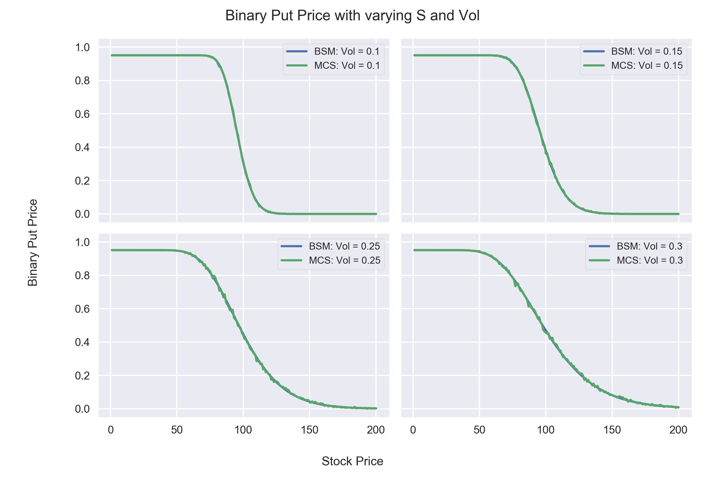
Observations:
From the above two set of graphs we can infer the following:
- Increase in volatility has contrasting effect on Binary Option Prices.
- For OTM (Out of the money) Options, the price increases, as higher volatility implies a greater chance of the option ending up in the money at expiry.
- For ITM (In the money) Options, the price decreases, as higher volatility implies a greater chance of the option ending up out of the money at expiry.
- This behaviour is different from that of a European Call Option whose value increases with higher volatility irrespctive of the option being ITM or OTM. This is because, for a Binary Option the upside is fixed and thus an ITM option would not benefit from higher volatility.
# Option Prices for different Stock Prices (S) and Risk Free Rate (R)
stockPrices = S.size
rCount = len(r)

BSCallR= np.zeros((stockPrices,rCount))
BSPutR = np.zeros((stockPrices,rCount))
MCCallR = np.zeros((stockPrices,rCount))
MCPutR = np.zeros((stockPrices,rCount))

for j,riskFree in enumerate(r):
    for i,s in np.ndenumerate(S):
        BSCallR[i,j] = BSValue(s,kDefault,tDefault,riskFree,volDefault,'Call')
        BSPutR[i,j] = BSValue(s,kDefault,tDefault,riskFree,volDefault,'Put')
        MCCallR[i,j] = MCValue(s,kDefault,tDefault,riskFree,volDefault,'Call',mDefault,nDefault)
        MCPutR[i,j] = MCValue(s,kDefault,tDefault,riskFree,volDefault,'Put',mDefault,nDefault)
print('Calculations Done')
# Plotting Results of MCS for Binary Call for different S and R

image_name = 'image7.png'       # Name of the Image File
image_path = os.path.join(images_folder_path, image_name)
fig, ((ax1,ax2),(ax3,ax4)) = plt.subplots(2,2,sharex = True, sharey = True)
axs = [ax1,ax2,ax3,ax4]
for i,ax in enumerate(axs):

    ax.plot(S,BSCallR[:,i], label='BSM: r = {}'.format(r[i]))
    ax.plot(S,MCCallR[:,i], label='MCS: r = {}'.format(r[i]))
    ax.set_ylim(-0.05,1.05)
    ax.tick_params(labelsize=9)
    ax.legend(fontsize=8,frameon=True)

fig.text(0.5, 0.04, 'Stock Price', ha='center')
fig.text(0.04, 0.5, 'Binary Call Price', va='center', rotation='vertical')
fig.suptitle("Binary Call Price with varying S and Risk-Free Rate",ha='center')
fig.subplots_adjust(left = 0.14,top=0.92, bottom = 0.14);
plt.savefig(image_path, dpi=300)
plt.close();
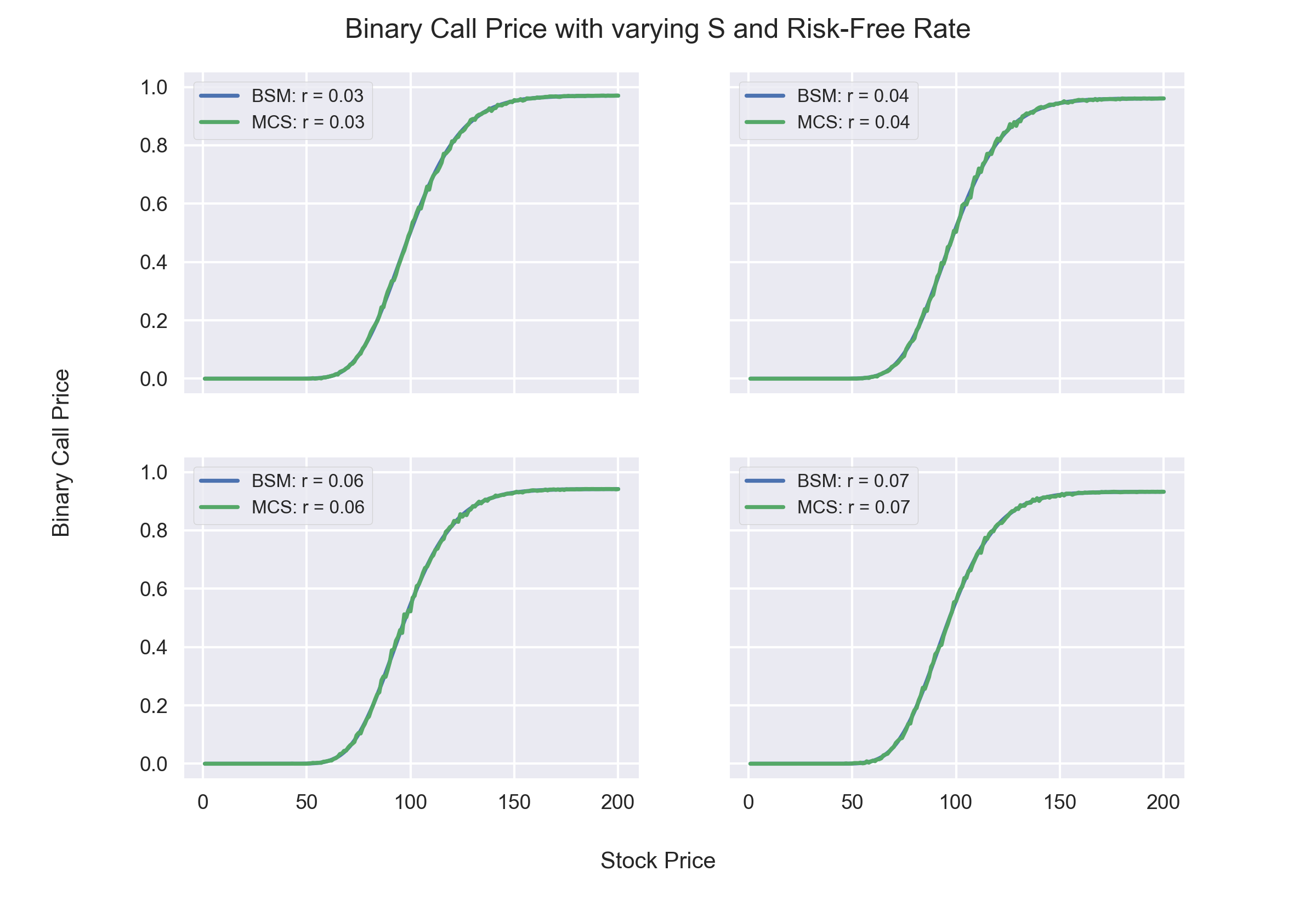
Observations:
- Binary Call Option Prices increase as Risk-Free rates increases
# Plotting Results of MCS for Binary Put for different S and R

image_name = 'image8.png'       # Name of the Image File
image_path = os.path.join(images_folder_path, image_name)
fig, ((ax1,ax2),(ax3,ax4)) = plt.subplots(2,2,sharex = True, sharey = True)
axs = [ax1,ax2,ax3,ax4]
for i,ax in enumerate(axs):

    ax.plot(S,BSPutR[:,i], label='BSM: r = {}'.format(r[i]))
    ax.plot(S,MCPutR[:,i], label='MCS: r = {}'.format(r[i]))
    ax.set_ylim(-0.05,1.05)
    ax.tick_params(labelsize=9)
    ax.legend(fontsize=8,frameon=True)

fig.text(0.5, 0.04, 'Stock Price', ha='center')
fig.text(0.04, 0.5, 'Binary Put Price', va='center', rotation='vertical')
fig.suptitle("Binary Put Price with varying S and Risk-Free Rate",ha='center')
fig.subplots_adjust(left = 0.14,top=0.92, bottom = 0.14);
plt.savefig(image_path, dpi=300)
plt.close();
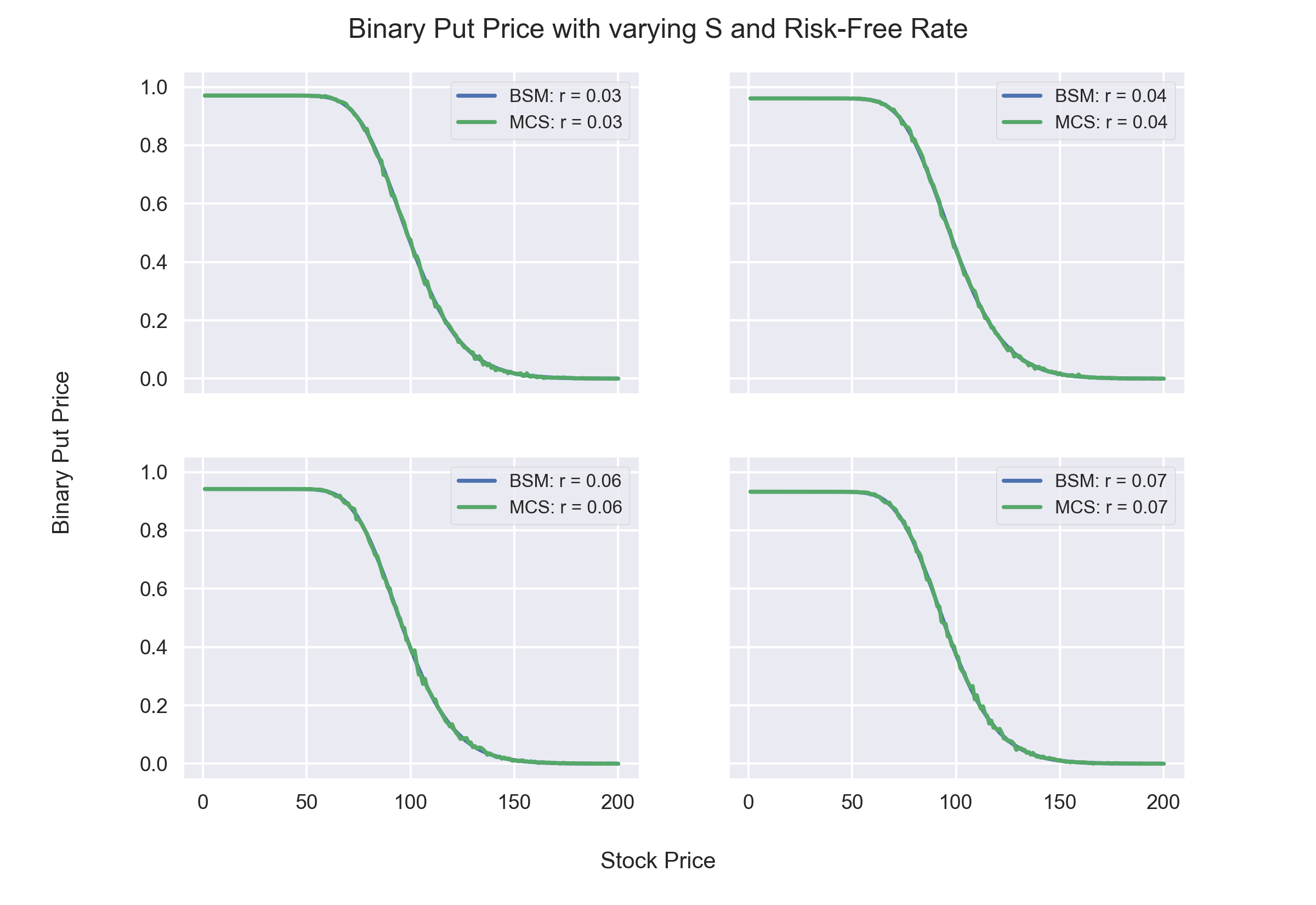
Observations:
- Binary Put Option Prices decrease as Risk-Free rates increases
#  Option Prices for different Stock Prices (S) and Time to maturity (T)

stockPrices = S.size
tCount = len(T)

BSCallT = np.zeros((stockPrices,tCount))
BSPutT = np.zeros((stockPrices,tCount))
MCCallT = np.zeros((stockPrices,tCount))
MCPutT = np.zeros((stockPrices,tCount))

for j,t in enumerate(T):
    for i,s in np.ndenumerate(S):
        BSCallT[i,j] = BSValue(s,kDefault,t,rDefault,volDefault,'Call')
        BSPutT[i,j] = BSValue(s,kDefault,t,rDefault,volDefault,'Put')
        MCCallT[i,j] = MCValue(s,kDefault,t,rDefault,volDefault,'Call',mDefault,nDefault)
        MCPutT[i,j] = MCValue(s,kDefault,t,rDefault,volDefault,'Put',mDefault,nDefault)
print('Calculations Done')
# Plotting Results of MCS for Binary Call for different S and T

image_name = 'image9.png'       # Name of the Image File
image_path = os.path.join(images_folder_path, image_name)
fig, ((ax1,ax2),(ax3,ax4)) = plt.subplots(2,2,sharex = True, sharey = True)
axs = [ax1,ax2,ax3,ax4]
for i,ax in enumerate(axs):

    ax.plot(S,BSCallT[:,i], label='BSM: T = {}'.format(T[i]))
    ax.plot(S,MCCallT[:,i], label='MCS: T = {}'.format(T[i]))
    ax.set_ylim(-0.05,1.05)
    ax.tick_params(labelsize=9)
    ax.legend(fontsize=8,frameon=True)

fig.text(0.5, 0.04, 'Stock Price', ha='center')
fig.text(0.04, 0.5, 'Binary Call Price', va='center', rotation='vertical')
fig.suptitle("Binary Call Price with varying S and Time to Maturity",ha='center')
fig.subplots_adjust(left = 0.14,top=0.92, bottom = 0.14);
plt.savefig(image_path, dpi=300)
plt.close();
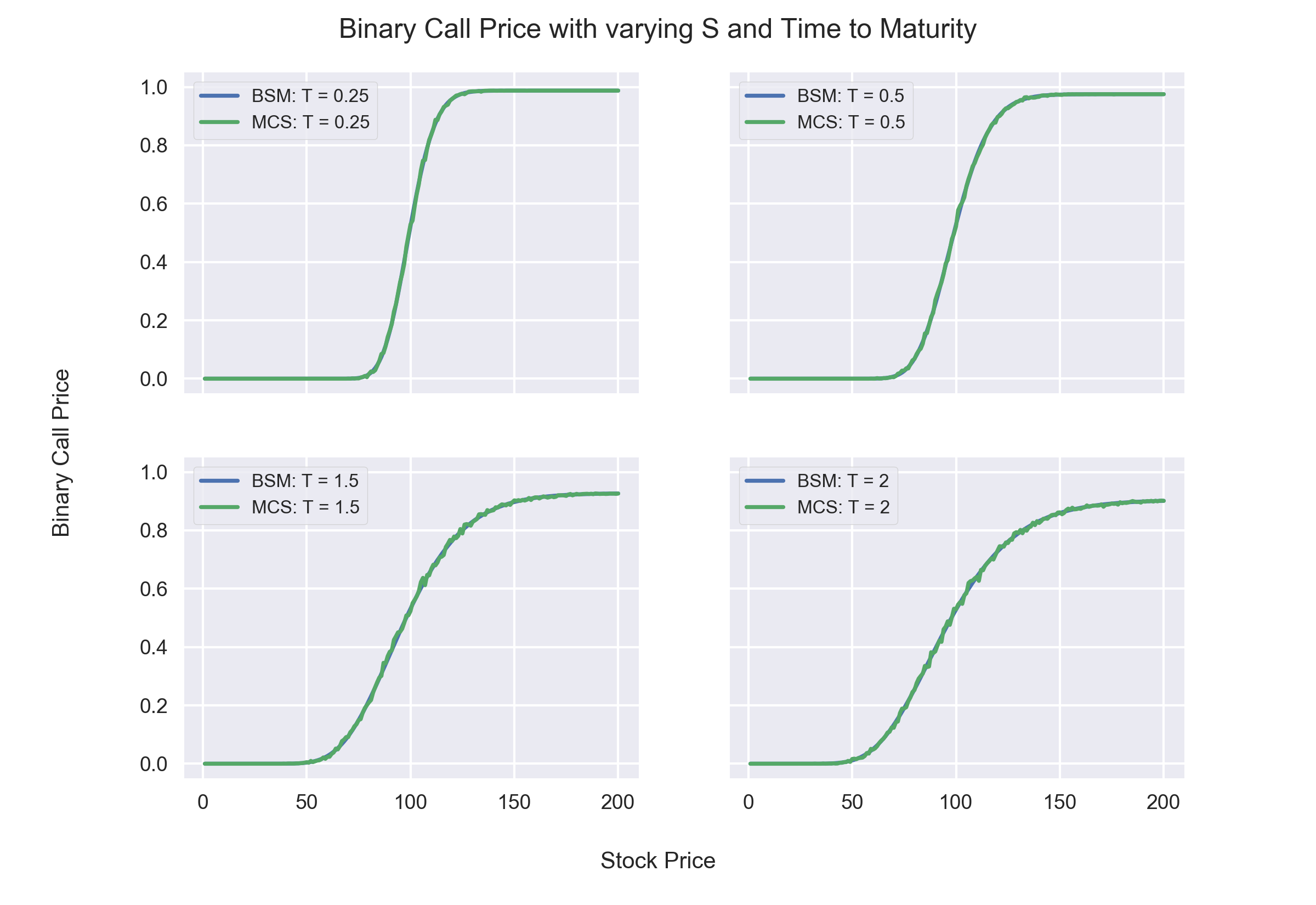
Observations:
- Price of OTM Binary Calls increase as Time to Maturity increases because time period for ending up in the money increases.
- Price of ITM Binary Calls decrease as Time to Maturity increases because time period for ending up out of the money increases.
# Plotting Results of MCS for Binary Put for different S and T

image_name = 'image10.png'       # Name of the Image File
image_path = os.path.join(images_folder_path, image_name)
fig, ((ax1,ax2),(ax3,ax4)) = plt.subplots(2,2,sharex = True, sharey = True)
axs = [ax1,ax2,ax3,ax4]
for i,ax in enumerate(axs):

    ax.plot(S,BSPutT[:,i], label='BSM: T = {}'.format(T[i]))
    ax.plot(S,MCPutT[:,i], label='MCS: T = {}'.format(T[i]))
    ax.set_ylim(-0.05,1.05)
    ax.tick_params(labelsize=9)
    ax.legend(fontsize=8,frameon=True)

fig.text(0.5, 0.04, 'Stock Price', ha='center')
fig.text(0.04, 0.5, 'Binary Put Price', va='center', rotation='vertical')
fig.suptitle("Binary Put Price with varying S and Time to Maturity",ha='center')
fig.subplots_adjust(left = 0.14,top=0.92, bottom = 0.14);
plt.savefig(image_path, dpi=300)
plt.close();
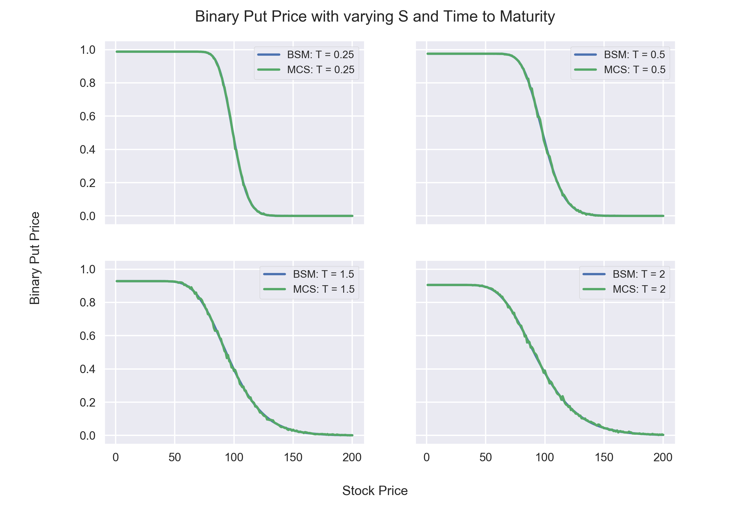
Observations:
- Price of OTM Binary Puts increase as Time to Maturity increases because time period for ending up in the money increases.
- Price of ITM Binary Puts decrease as Time to Maturity increases because time period for ending up out of the money increases.
- However, the effect of Time to Maturity is complicated on Binary Puts. This is because on one hand the longer Time to Maturity increases volatility, which increases the Put's value, on the other hand it decreases the present value of the payoff, which decreases the Put's value.
# Option Prices for ATM,ITM and OTM Call and Puts for Varying Vol

sRange = [90,100,110]
stockPrices = len(sRange)
nVol = 100
volRange = np.linspace(0.01,0.6,nVol)
BSCallVolRa = np.zeros((nVol,stockPrices))
BSPutVolRa = np.zeros((nVol,stockPrices))
MCCallVolRa = np.zeros((nVol, stockPrices))
MCPutVolRa = np.zeros((nVol, stockPrices))

for j,s in enumerate(sRange):
    for i,sigma in np.ndenumerate(volRange):
            BSCallVolRa[i,j] = BSValue(s,kDefault,tDefault,rDefault,sigma,'Call')
            BSPutVolRa[i,j] = BSValue(s,kDefault,tDefault,rDefault,sigma,'Put')
            MCCallVolRa[i,j] = MCValue(s,kDefault,tDefault,rDefault,sigma,'Call',mDefault,nDefault)
            MCPutVolRa[i,j] = MCValue(s,kDefault,tDefault,rDefault,sigma,'Put',mDefault,nDefault)
print('Calculations Done')
# Plotting Option Prices for ATM,ITM and OTM Call and Puts for Varying Vol

image_name = 'image11.png'       # Name of the Image File
image_path = os.path.join(images_folder_path, image_name)
fig, ((ax1,ax2),(ax3,ax4),(ax5,ax6)) = plt.subplots(3,2,sharex = True,sharey=True,figsize=(8,8))
axCall = [ax1,ax3,ax5]
axPut = [ax2,ax4,ax6]

for i,ax in enumerate(axCall):

    ax.plot(volRange,BSCallVolRa[:,i], label='BSM: S = {}'.format(sRange[i]))
    ax.plot(volRange,MCCallVolRa[:,i], label='MCS: S = {}'.format(sRange[i]))
    ax.set_ylim(-0.05,1.05)
    ax.tick_params(labelsize=9)
    ax.legend(fontsize=8,frameon=True)

for i,ax in enumerate(axPut):

    ax.plot(volRange,BSPutVolRa[:,i], label='BSM: S = {}'.format(sRange[i]))
    ax.plot(volRange,MCPutVolRa[:,i], label='MCS: S = {}'.format(sRange[i]))
    ax.set_ylim(-0.05,1.05)
    ax.tick_params(labelsize=9)
    ax.legend(fontsize=8,frameon=True)

ax1.set_title("Binary Call")
ax2.set_title("Binary Put")
fig.text(0.5, 0.04, 'Volatility', ha='center')
fig.text(0.04, 0.5, 'Binary Option Price', va='center', rotation='vertical')
fig.suptitle("Binary Option Price with varying Volatility, K = 100",ha='center')
fig.subplots_adjust(left = 0.14,top=0.88, bottom = 0.14);
plt.savefig(image_path, dpi=300)
plt.close();
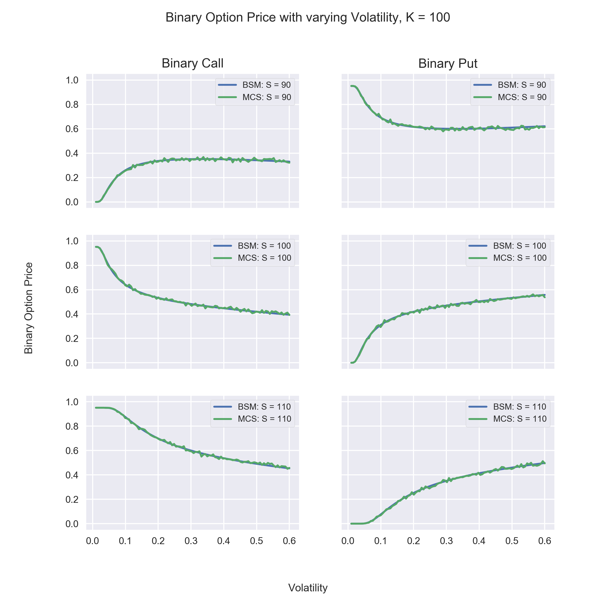
Observations:
- Price of OTM Options increases as volatility increases.
- Price of ITM Options decrease as volatility increases.
# Option Prices for ATM,ITM and OTM Call and Puts for Varying Risk Free Rate

sRange = [90,100,110]
stockPrices = len(sRange)
nR = 100
rRange = np.linspace(0.01,0.2,nR)
BSCallrRa = np.zeros((nR,stockPrices))
BSPutrRa = np.zeros((nR,stockPrices))
MCCallrRa = np.zeros((nR,stockPrices))
MCPutrRa = np.zeros((nR,stockPrices))

for j,s in enumerate(sRange):
    for i,r in np.ndenumerate(rRange):
            BSCallrRa[i,j] = BSValue(s,kDefault,tDefault,r,volDefault,'Call')
            BSPutrRa[i,j] = BSValue(s,kDefault,tDefault,r,volDefault,'Put')
            MCCallrRa[i,j] = MCValue(s,kDefault,tDefault,r,volDefault,'Call',mDefault,nDefault)
            MCPutrRa[i,j] = MCValue(s,kDefault,tDefault,r,volDefault,'Put',mDefault,nDefault)
print('Calculations Done')
# Plotting Option Prices for ATM,ITM and OTM Call and Puts for Varying Risk-Free Rate

image_name = 'image12.png'       # Name of the Image File
image_path = os.path.join(images_folder_path, image_name)

fig, ((ax1,ax2),(ax3,ax4),(ax5,ax6)) = plt.subplots(3,2,sharex = True,sharey=True, figsize=(8,8))
axCall = [ax1,ax3,ax5]
axPut = [ax2,ax4,ax6]

for i,ax in enumerate(axCall):

    ax.plot(rRange,BSCallrRa[:,i], label='BSM: S = {}'.format(sRange[i]))
    ax.plot(rRange,MCCallrRa[:,i], label='MCS: S = {}'.format(sRange[i]))
    ax.set_ylim(-0.05,1.05)
    ax.set_xlim(-0.01,0.21)
    ax.tick_params(labelsize=9)
    ax.legend(fontsize=8,frameon=True)

for i,ax in enumerate(axPut):

    ax.plot(rRange,BSPutrRa[:,i], label='BSM: S = {}'.format(sRange[i]))
    ax.plot(rRange,MCPutrRa[:,i], label='MCS: S = {}'.format(sRange[i]))
    ax.set_ylim(-0.05,1.05)
    ax.set_xlim(-0.01,0.21)
    ax.tick_params(labelsize=9)
    ax.legend(fontsize=8,frameon=True)

ax1.set_title("Binary Call")
ax2.set_title("Binary Put")
fig.text(0.5, 0.04, 'Risk-Free Rate', ha='center')
fig.text(0.04, 0.5, 'Binary Option Price', va='center', rotation='vertical')
fig.suptitle("Binary Option Price with varying Risk Free Rate, K = 100",ha='center')
fig.subplots_adjust(left = 0.14,top=0.88, bottom = 0.14);
plt.savefig(image_path, dpi=300)
plt.close();
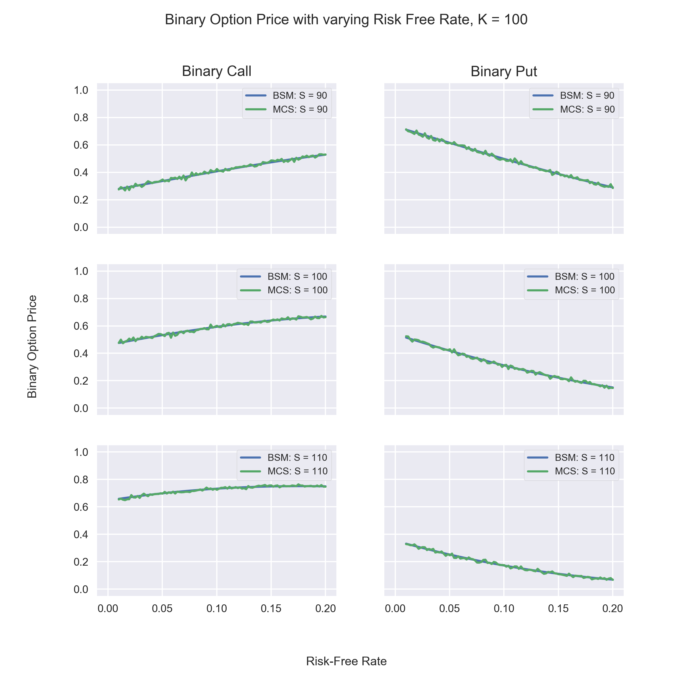
Observations:
- Call Prices increase as Risk-Free Rate increases.
- Put Prices decrease as Risk-Free Rate increases.
# Option Prices for ATM,ITM and OTM Call and Puts for Varying Time to Maturity

sRange = [90,100,110]
stockPrices = len(sRange)
tR = 100
tRange = np.linspace(0.1,2,tR)
BSCalltRa = np.zeros((tR,stockPrices))
BSPuttRa = np.zeros((tR,stockPrices))
MCCalltRa = np.zeros((tR,stockPrices))
MCPuttRa = np.zeros((tR,stockPrices))

for j,s in enumerate(sRange):
    for i,t in np.ndenumerate(tRange):
            BSCalltRa[i,j] = BSValue(s,kDefault,t,rDefault,volDefault,'Call')
            BSPuttRa[i,j] = BSValue(s,kDefault,t,rDefault,volDefault,'Put')
            MCCalltRa[i,j] = MCValue(s,kDefault,t,rDefault,volDefault,'Call',mDefault,nDefault)
            MCPuttRa[i,j] = MCValue(s,kDefault,t,rDefault,volDefault,'Put',mDefault,nDefault)
print('Calculations Done')
# Plotting Option Prices for ATM,ITM and OTM Call and Puts for Varying Time to Maturtiy

image_name = 'image13.png'       # Name of the Image File
image_path = os.path.join(images_folder_path, image_name)
fig, ((ax1,ax2),(ax3,ax4),(ax5,ax6)) = plt.subplots(3,2,sharex = True,sharey=True, figsize=(8,8))
axCall = [ax1,ax3,ax5]
axPut = [ax2,ax4,ax6]

for i,ax in enumerate(axCall):

    ax.plot(tRange,BSCalltRa[:,i], label='BSM: S = {}'.format(sRange[i]))
    ax.plot(tRange,MCCalltRa[:,i], label='MCS: S = {}'.format(sRange[i]))
    ax.set_ylim(-0.05,1.05)
    ax.set_xlim(0.1,2.05)
    ax.tick_params(labelsize=9)
    ax.legend(fontsize=8,frameon=True)

for i,ax in enumerate(axPut):

    ax.plot(tRange,BSPuttRa[:,i], label='BSM: S = {}'.format(sRange[i]))
    ax.plot(tRange,MCPuttRa[:,i], label='MCS: S = {}'.format(sRange[i]))
    ax.set_ylim(-0.05,1.05)
    ax.set_xlim(-0.1,2.05)
    ax.tick_params(labelsize=9)
    ax.legend(fontsize=8,frameon=True)

ax1.set_title("Binary Call")
ax2.set_title("Binary Put")
fig.text(0.5, 0.04, 'Time to Maturity', ha='center')
fig.text(0.04, 0.5, 'Binary Option Price', va='center', rotation='vertical')
fig.suptitle("Binary Option Price with varying Time to Maturity, K = 100",ha='center')
fig.subplots_adjust(left = 0.14,top=0.88, bottom = 0.14);
plt.savefig(image_path, dpi=300)
plt.close();
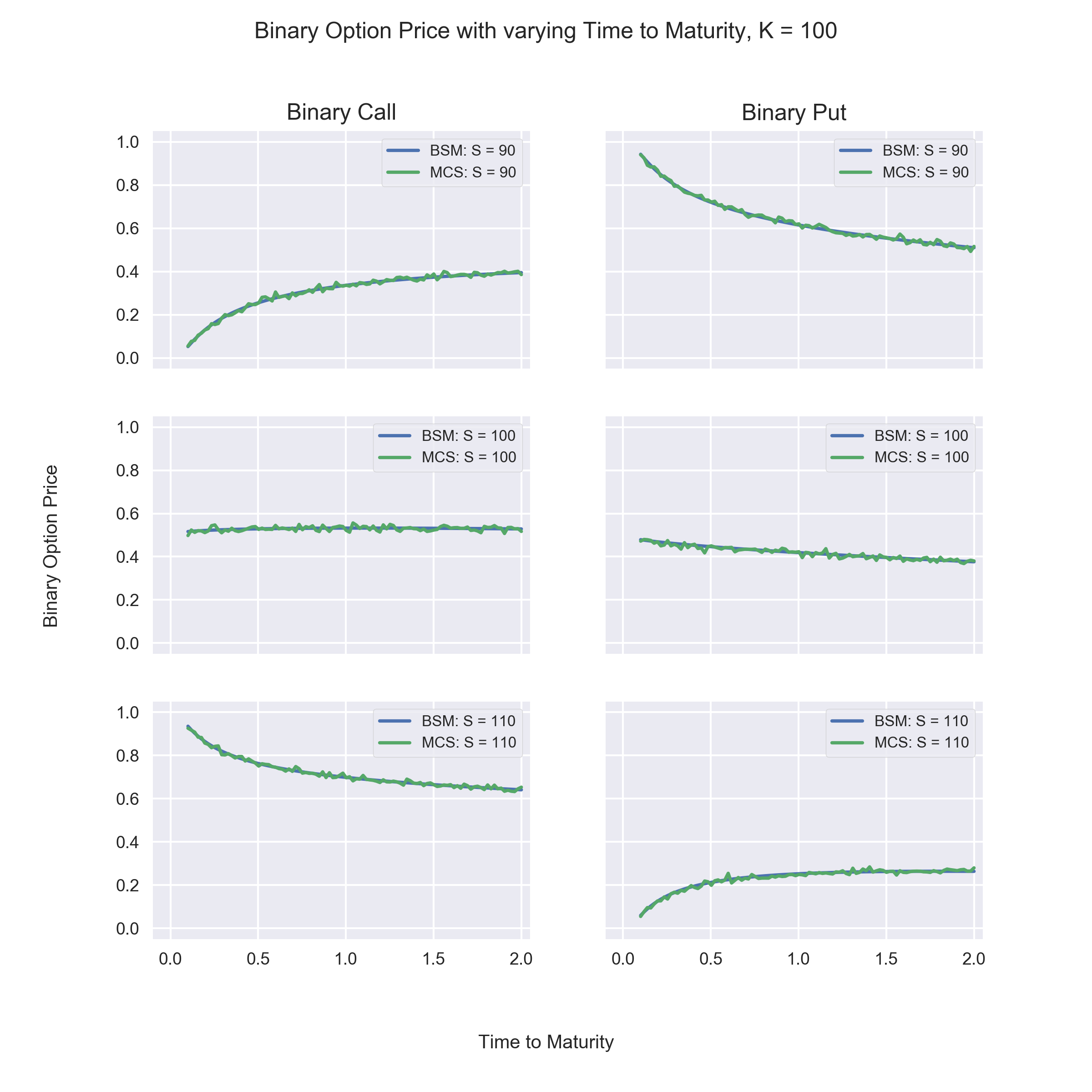
Observations:
- The increase in OTM Call Option's price is faster than the increase in OTM Put Option's price as Time to Maturity increases.
- The decrease in ITM Call Options's price is slower than the decrease in ITM Put Options' price as Time to Maturity increases.
- The above is due to two different factors affecting the Put Value in opposite directions. On one hand the longer Time to Maturity increases volatility, which increases the Put's value, on the other hand it decreases the present value of the payoff, which decreases the Put's value.
Conclusion:
Binary Options have been priced using both Monte Carlo Simulations and Black Scholes Model. Then, Binary Option Prices have been analysed with respect to varying Stock Prices, Volatility, Risk-Free Rate and Time to Maturity.
- Higher number of Time Steps and Simulations increase the accuracy of Monte Carlo Simulations.
- Magnitude of Delta is highest when Stock Price is close to the Strike Price.
- Volatility increases the price of OTM Options but it decreases the price of ITM Options.
- Higher the Risk-Free Rate, higher the Call Option Price and lower the Put Option Price.
- As Time to Maturity increases, OTM Call Option Price increases and ITM Call Option Price decreases.
- Effect of Time to Maturity on Put Option Price is more complex and depends on the interplay of Risk-Free rate, volatility and Time to Maturity.
References:
Euler-Maruyama Method:
- https://www.stat.berkeley.edu/~arturof/Teaching/STAT150/Notes/II_Brownian_Motion.pdf
- http://www.math.kit.edu/ianm3/lehre/nummathfin2012w/media/euler_maruyama.pdf
- https://ipython-books.github.io/134-simulating-a-stochastic-differential-equation/
- http://www.mecs-press.org/ijisa/ijisa-v8-n6/IJISA-V8-N6-6.pdf
Option Pricing:
- Wilmott P.(2018). Paul Wilmott Introduces Quantitative Finance, 2nd Edition
- http://konvexity.com/factors-affecting-value-of-an-option
- https://quant.stackexchange.com/questions/16064/effect-of-time-to-maturity-on-european-put-option
- https://binarytradingclub.com/binary-option-pricing/
- https://www.nadex.com/learning-center/glossary/what-does-volatility-mean
- https://breakingdownfinance.com/finance-topics/derivative-valuation/option-valuation/binary-option-pricing/
- https://financetrain.com/impact-of-exercise-price-and-time-to-expiry-on-option-prices/
Python Coding and Latex Typing in Jupyter Notebook:
- Hilpisch Y.(2018). Python for Finance, 2nd Edition
- CQF Pre Course Resources, Introduction to Python Primer
- https://daringfireball.net/projects/markdown/
- https://www.math.ubc.ca/~pwalls/math-python/jupyter/latex/#common-symbols