Assignment - Module 3
30 July 2021
Group 23: Aman Jindal | Yuhang Jiang | Daniel Gabriel Tan | Qining Liu
# Importing Libraries

import pandas as pd
import numpy as np
from pprint import pprint
from functools import reduce
import dateparser
import matplotlib.pyplot as plt
plt.style.use('seaborn')
Q1. List Comprehension: First generate a list using the range(20) function. Next, create a second list that calculates 0.5 ⋅ n ⋅ (n+1) for each item n in the first list. Solve this using a while loop and also the list comprehension method. Check if the outputs match for the two methods.
Answer 1:
# While Loop Method

input_list = range(20)
ans_q1_whileLoop = []
i = 0
while i < len(input_list):
    ans_q1_whileLoop.append(0.5*input_list[i]*(input_list[i]+1))
    i = i + 1

print('Answer:\n\n {}'.format(ans_q1_whileLoop))
print('\nLength of the list: {}'.format(len(ans_q1_whileLoop)))
Answer:

 [0.0, 1.0, 3.0, 6.0, 10.0, 15.0, 21.0, 28.0, 36.0, 45.0, 55.0, 66.0, 78.0, 91.0, 105.0, 120.0, 136.0, 153.0, 171.0, 190.0]

Length of the list: 20
# List Comprehension Method

input_list = range(20)
ans_q1_lc = [0.5*n*(n+1) for n in input_list]

print('Answer:\n\n {}'.format(ans_q1_lc))
print('\nLength of the list: {}'.format(len(ans_q1_lc)))
Answer:

 [0.0, 1.0, 3.0, 6.0, 10.0, 15.0, 21.0, 28.0, 36.0, 45.0, 55.0, 66.0, 78.0, 91.0, 105.0, 120.0, 136.0, 153.0, 171.0, 190.0]

Length of the list: 20
# Check if the two lists are equal

print('Check if the lists are equal: {}'.format(ans_q1_whileLoop == ans_q1_lc))
Check if the lists are equal: True
Q2. Lambda function: Create a numpy array of integers from 1 to 50. Use the lambda function to compute x3 + x2 + x + 1 for each element x of the array. Compare your output using the list comprehension method.
Answer 2:
# A General Purpose Function for calculating sum of a geometric power series where a = 1 & r = pow

def sum_geom_pow(elem, pow): return sum([elem**p for p in range(pow+1)])
# Lambda Function Method

input_arr = np.arange(50)+1
max_pow = 3

cubic_func = lambda x: sum_geom_pow(x, max_pow)
ans_q2_lambda = cubic_func(input_arr)
print('Answer:\n')
pprint(ans_q2_lambda)
Answer:

array([     4,     15,     40,     85,    156,    259,    400,    585,
          820,   1111,   1464,   1885,   2380,   2955,   3616,   4369,
         5220,   6175,   7240,   8421,   9724,  11155,  12720,  14425,
        16276,  18279,  20440,  22765,  25260,  27931,  30784,  33825,
        37060,  40495,  44136,  47989,  52060,  56355,  60880,  65641,
        70644,  75895,  81400,  87165,  93196,  99499, 106080, 112945,
       120100, 127551], dtype=int32)
# List Comprehension Method

input_arr = np.arange(50)+1
max_pow = 3

ans_q2_lc = np.array([sum_geom_pow(x, max_pow) for x in input_arr])
print('Answer:\n')
pprint(ans_q2_lc)
Answer:

array([     4,     15,     40,     85,    156,    259,    400,    585,
          820,   1111,   1464,   1885,   2380,   2955,   3616,   4369,
         5220,   6175,   7240,   8421,   9724,  11155,  12720,  14425,
        16276,  18279,  20440,  22765,  25260,  27931,  30784,  33825,
        37060,  40495,  44136,  47989,  52060,  56355,  60880,  65641,
        70644,  75895,  81400,  87165,  93196,  99499, 106080, 112945,
       120100, 127551])
# Check if the two outputs are equal

print('Check if the arrays are equal: {}'.format((ans_q2_lambda == ans_q2_lc).all()))
Check if the arrays are equal: True
Q3. For Loop: Create a list with range(50). Return x3 + x2 + x + 1 for every element x in the list with an exception that for the last 5 elements return x4 + x3 + x2 + x + 1. Use a for loop to do this operation. Hint: You might want to read up on “enumerate” and how that can be used with a for loop.
Answer 3:
# For Loop Method

input_list = range(50)
last_elem_count = 5
max_pow_start45 = 3
max_pow_last5 = 4
ans_q3_forLoop = []

for i, x in enumerate(input_list):
    if i >= len(input_list)-last_elem_count:
        ans_q3_forLoop.append(sum_geom_pow(x, max_pow_last5))
    else:
        ans_q3_forLoop.append(sum_geom_pow(x, max_pow_start45))

print('Answer: \n\n{}'.format(ans_q3_forLoop))
Answer:

[1, 4, 15, 40, 85, 156, 259, 400, 585, 820, 1111, 1464, 1885, 2380, 2955, 3616, 4369, 5220, 6175, 7240, 8421, 9724, 11155, 12720, 14425, 16276, 18279, 20440, 22765, 25260, 27931, 30784, 33825, 37060, 40495, 44136, 47989, 52060, 56355, 60880, 65641, 70644, 75895, 81400, 87165, 4193821, 4576955, 4985761, 5421361, 5884901]
# List Comprehension Method

input_list = range(50)
last_elem_count = 5
max_pow_start45 = 3
max_pow_last5 = 4

ans_q3_lc = [sum_geom_pow(x, max_pow_last5)
             if i >= len(input_list)-last_elem_count
             else sum_geom_pow(x, max_pow_start45)
             for i, x in enumerate(input_list)]

print('Answer: \n\n{}'.format(ans_q3_lc))
Answer:

[1, 4, 15, 40, 85, 156, 259, 400, 585, 820, 1111, 1464, 1885, 2380, 2955, 3616, 4369, 5220, 6175, 7240, 8421, 9724, 11155, 12720, 14425, 16276, 18279, 20440, 22765, 25260, 27931, 30784, 33825, 37060, 40495, 44136, 47989, 52060, 56355, 60880, 65641, 70644, 75895, 81400, 87165, 4193821, 4576955, 4985761, 5421361, 5884901]
# Check if the two outputs are equal

print('Check if the arrays are equal: {}'.format((ans_q3_forLoop == ans_q3_lc)))
Check if the arrays are equal: True
Q4. List comprehension with logical statements: First generate a list using the range(30) function. Next, create a second list that creates elements based on the logic below. Hint: You can do this by including an if statement inside your list comprehension.
f(x) = x2, if x is even;
f(x) = x3, if x is odd.
Answer 4:
input_list = range(30)

ans_q4 = [x**2 if x % 2 == 0 else x**3 for x in input_list]

print('Answer: \n\n{}'.format(ans_q4))
Answer:

[0, 1, 4, 27, 16, 125, 36, 343, 64, 729, 100, 1331, 144, 2197, 196, 3375, 256, 4913, 324, 6859, 400, 9261, 484, 12167, 576, 15625, 676, 19683, 784, 24389]
Q5. Fibonacci sequence: Construct a function “fibonacci” that takes in the required variable integer “n” and returns the nt**h term in a Fibonacci sequence (1,1,2,3,5,…). For example, if your call your function and pass in the argument n = 6, i.e fibonacci(n=6) it should return the value 8. You can use a for or a while loop inside your function. Print the function output for n=30, 50, and 100.
Answer 5:
# Method 1 of generating the nth element of the Fibonacci series

pos_list = [6, 30, 50, 100]

def get_fib_nth_elem_m1(elem_pos=0):
    if isinstance(elem_pos, int) and elem_pos >= 0:
        return reduce(lambda x, _:(x[1],x[0]+x[1]), range(elem_pos), (0,1))[0]
    else:
        raise TypeError('Element Position entered is not an integer greater than or equal to 0')

for pos in pos_list:
   print('Fibonacci Series Value at position {}: {:,}\n'.format(pos, get_fib_nth_elem_m1(pos)))
Fibonacci Series Value at position 6: 8

Fibonacci Series Value at position 30: 832,040

Fibonacci Series Value at position 50: 12,586,269,025

Fibonacci Series Value at position 100: 354,224,848,179,261,915,075
# Method 2 of generating the nth element of the Fibonacci series

pos_list = [6, 30, 50, 100]

def get_fib_nth_elem_m2(elem_pos=0):

    if isinstance(elem_pos, int) and elem_pos >= 0:
        a, b = 0, 1
        for i in range(elem_pos):
            a, b = b, a+b
        return a
    else:
        raise TypeError('Element Position entered is not an integer greater than or equal to 0')

for pos in pos_list:
 print('Fibonacci Series Value at position {}: {:,}\n'.format(pos, get_fib_nth_elem_m2(pos)))
Fibonacci Series Value at position 6: 8

Fibonacci Series Value at position 30: 832,040

Fibonacci Series Value at position 50: 12,586,269,025

Fibonacci Series Value at position 100: 354,224,848,179,261,915,075
# Method 3 of generating the nth element of the Fibonacci series

from functools import lru_cache
pos_list = [6, 30, 50, 100]

@lru_cache(maxsize=1000)
def get_fib_nth_elem_m3(n):
    """Function takes input integer 'n' and returns the n-th sequence of the fibonacci series
       (no loops & no memoization)"""

    if n <= 2 : return 1
    else : return get_fib_nth_elem_m3(n-1) + get_fib_nth_elem_m3(n-2)

for pos in pos_list:
   print('Fibonacci Series Value at position {}: {:,}\n'.format(pos, get_fib_nth_elem_m3(pos)))
Fibonacci Series Value at position 6: 8

Fibonacci Series Value at position 30: 832,040

Fibonacci Series Value at position 50: 12,586,269,025

Fibonacci Series Value at position 100: 354,224,848,179,261,915,075
Q6. Net Present Value: Code up a function that computes the net present value of a stream of cash-flows and call this function NPV. The function will take three inputs - cash-flows, dates, and interest rate (constant). We will use the formula specified below to compute the NPV of a stream of cash-flows on specific dates. The time periods t1, t2, .., tN are computed as differences from first date. Make sure you annualize the difference in days (convert them to years). Check out this wikipedia link if you want to read up some more.
Run this function for the following input:
Compute : NPV(CF=[-100,50,40,30], date=[01-Jan-2020,31-Mar-2021,30-Jun-2021,31-Dec-2024], r=0.05)
Answer 6:
Notes on Parsing Dates:
- Date Formats are available here for parsing string as dates
- dateparser library is a powerful library for parsing dates from strings. It can even parse dates without the assistance of a date format.
- Further, more than one date formats can also be supplied, as
elements of a list, to the
date_formatsargument ofdateparser.parsefunction.
def NPV(cash_flows, cf_dates, interest_rate):
    '''
    Computes the NPV of a series of cash flows. First date in the cf_dates list is assumed to
    be the NPV calculation date

    Args:
    cash_flows (list of int/float): List of cash flows
    cf_dates (list of str): List of cash flow dates in the str format 'DD-MMM-YYYY'
                            (e.g.: 01-Jan-2021)
    interest_rate (int/float): Yearly Interest Rate for discounting (absolute value)

    Returns:
    npv (float): Net Present Value of the cash flows
    '''


    date_formats = ['%d-%b-%Y']    # More date formats can be supplied as additional list elements
    days_a_year = 365              # Actual/365 day-count convetion is chosen

    cf_dates_parsed = [dateparser.parse(date_string=date_string,
                                        date_formats=date_formats).date()
                       for date_string in cf_dates]

    cf_time_deltas =  [(cf_date - cf_dates_parsed[0]).days/days_a_year
                       for cf_date in cf_dates_parsed]

    pv_cash_flows = [cash_flow/(1+interest_rate)**time_to_maturity
                     for cash_flow, time_to_maturity in zip(cash_flows, cf_time_deltas)]

    npv = sum(pv_cash_flows)
    return npv
cash_flows = [-100, 50, 40, 30]
cash_flow_dates = ['01-Jan-2020', '31-Mar-2021', '30-Jun-2021', '31-Dec-2024']
interest_rate = 0.05

print('NPV of the cash flows: {:,.2f}'.format(NPV(cash_flows, cash_flow_dates, interest_rate)))
NPV of the cash flows: 7.74
Q7. Pandas .rolling() is a very useful function to know (check out the doc string of pandas.Series.rolling for a better understanding of what the function does). In this problem, we will calculate the 1-year rolling sum of returns for the data in stock_data.csv file. Clean the data (remove strings and drop NaN values). Use the pandas rolling function (window=12) to calculate the sum of 1-year returns. Add this column to the original dataframe.
Answer 7:
# Setting the Input File Path

input_file_folder = 'Data'          # Folder Name within the cwd where the data file is stored
input_file_name = 'stock_data.csv'  # Name of the File
cwd = os.getcwd()
input_file_path = os.path.join(cwd, input_file_folder, input_file_name)
- More details on dtpyes & converters used below while reading data is available here
- In the above link, the comparison between specifying dtypes and specifying converters while using the pandas read function is quite useful
# Reading & Cleaning the Data

def numeric_converter(x): return pd.to_numeric(x, errors='coerce')

# Specifying dtype converters for specific columns
converters = {'total_returns': numeric_converter,
              'price': numeric_converter,
              'date': lambda x: pd.to_datetime(x, errors='coerce')}

df = pd.read_csv(filepath_or_buffer=input_file_path, sep=',', header=0,
                 converters=converters).dropna(axis=0, how='any').reset_index(drop=True)

df.drop_duplicates(subset=['permno', 'date'], keep='first', inplace=True, ignore_index=True)
df.sort_values(by = ['permno', 'date'], ascending=[True, True], inplace=True, ignore_index=True)
df.shape
(2913, 6)
# Calculating 12 months Rolling Returns & Adding them to the DataFrame

def calc_roll_returns(df, months=12):

    # Offset is 1 month less as the addition of returns is inclusive of both start & end months
    # Additional 10 days are added while comparing 11 month previous date to allow
    # for misaligned months such as Feb

    offset = months - 1
    df.reset_index(inplace=True, drop=True)
    return [np.nan if index < offset else np.nan if
            df.loc[index-offset, 'date'] < (df.loc[index, 'date']
            - pd.DateOffset(months=offset, days=10)) else
            sum([df_group.loc[i, 'total_returns'] for i in range(index-offset, index+1)])
            for index in df_group.index]

months = 12                     # Rolling returns required for 12 months
roll_returns = []
for _, df_group in df.groupby('permno'):
    roll_returns.extend(calc_roll_returns(df_group, 12))

df['roll_returns_'+str(months)+'months'] = roll_returns
print(df.tail())
      permno          company_name       date  total_returns  price  \
2908   10137  ALLEGHENY ENERGY INC 2010-07-31       0.102514  22.80
2909   10137  ALLEGHENY ENERGY INC 2010-08-31      -0.010965  22.55
2910   10137  ALLEGHENY ENERGY INC 2010-09-30       0.094013  24.52
2911   10137  ALLEGHENY ENERGY INC 2010-10-31      -0.053834  23.20
2912   10137  ALLEGHENY ENERGY INC 2011-01-31       0.063531  25.78

      share_outstanding  roll_returns_12months
2908             169579              -0.041395
2909             169615              -0.099960
2910             169615              -0.015792
2911             169615               0.069891
2912             169939                    NaN
Q8. Combining Pandas apply and lambda functions: Load and clean the stock_data.csv file. Compute the market cap by multiplying the price and outstanding shares. You need to segregate PERMNOs into large-cap, mid-cap, and small-cap stocks. First, you have to write a function that takes in a value x (market cap) as an input. For segregating use the following criteria mentioned below. Use the pandas apply along with lambda function, to pass the function pass you have just coded up.
f(x) = small cap, if x < 100000
f(x) = mid cap, 100000 ≤ if x < 1000000
f(x) = large cap, if x ≥ 1000000
Answer 8:
# For each permno, average market cap has been used yo determine market cap size

m_cap_types = ['small_cap', 'mid_cap', 'large_cap']

pd.options.display.float_format = '{:,.2f}'.format       # Setting Display Options for Market Cap

df['market_cap'] = df['price']*df['share_outstanding']
mcap_determiner = lambda x: np.select(condlist=
                            [x['market_cap']<10**5, x['market_cap']>10**6],
                            choicelist=['small_cap', 'large_cap'],
                                      default='mid_cap')

df_updated = df.groupby('permno')['market_cap'].mean().reset_index()\
               .assign(m_cap_size = lambda x: mcap_determiner(x))

m_cap_permno_dict = {m_cap_type:
                    df_updated.loc[df_updated['m_cap_size'] == m_cap_type, 'permno']
                              .unique().tolist()
                    for m_cap_type in m_cap_types}
print('Answer:\n\n{}'.format(m_cap_permno_dict))
Answer:

{'small_cap': [10001, 10014, 10028, 10029, 10042, 10057, 10066, 10097, 10116, 10125], 'mid_cap': [10006, 10048, 10051, 10064, 10071, 10085, 10092, 10102, 10120, 10123], 'large_cap': [10104, 10108, 10119, 10126, 10137]}
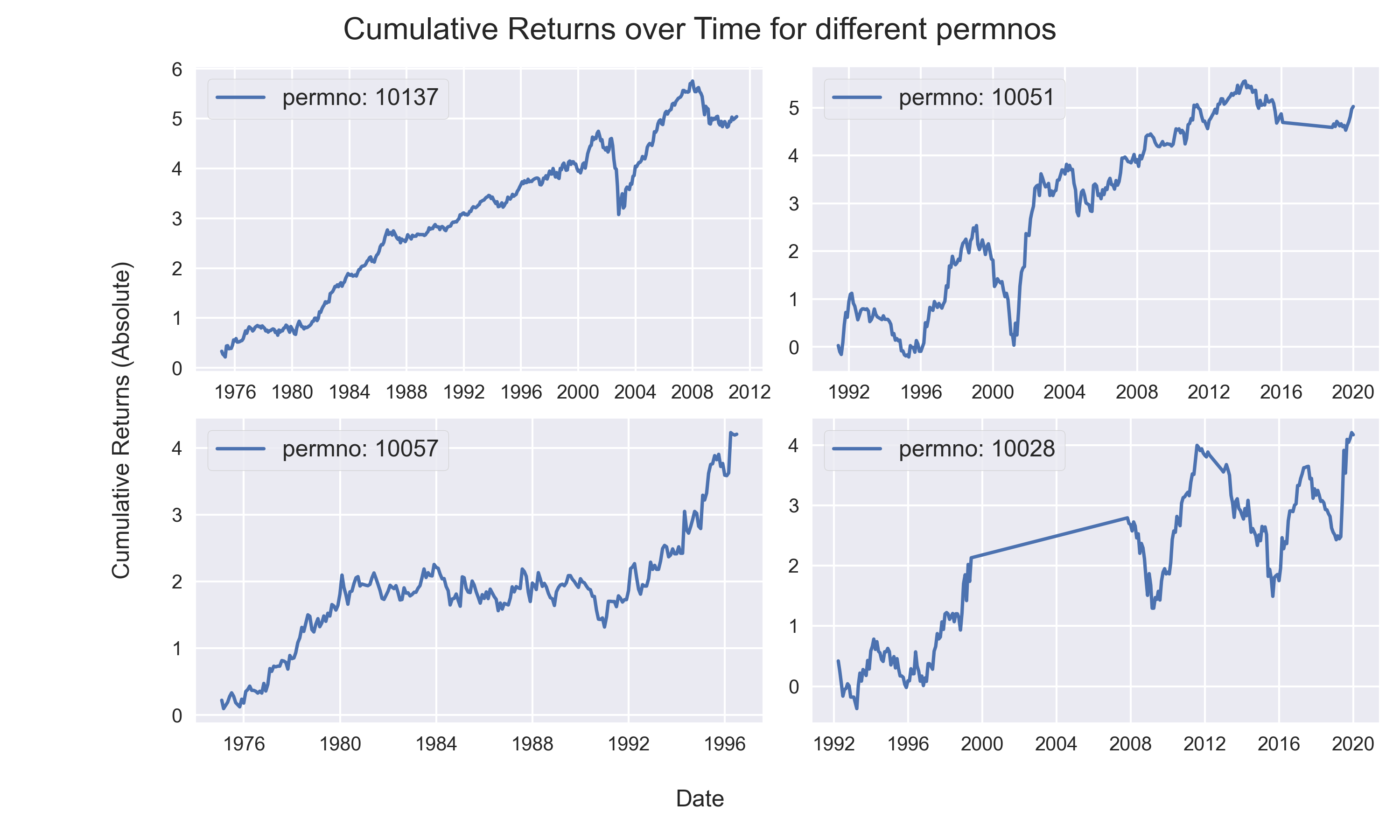
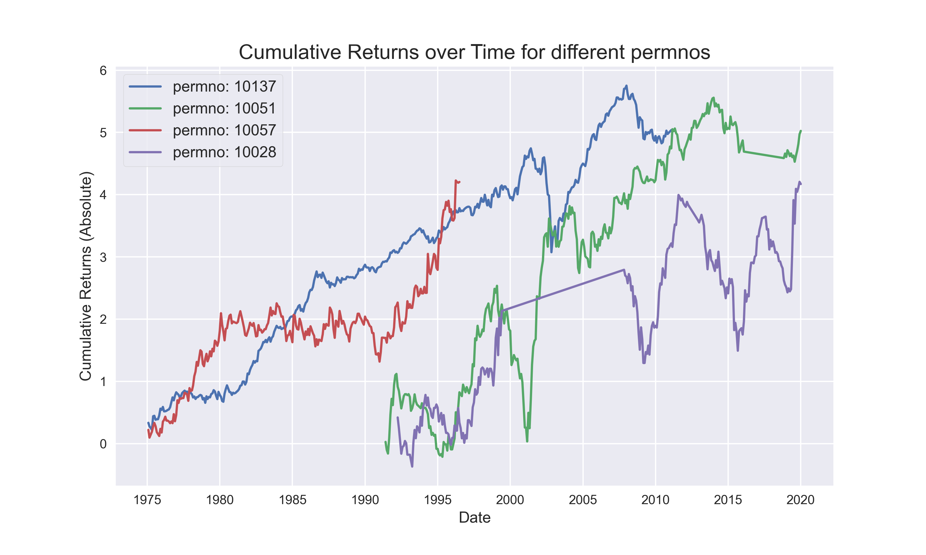
Q9.Plot and Subplots: For the 4 PERMNOs - (10137, 10051, 10057, 10028), calculate the cumulative sum of returns and plot them in a 4-by-4 sub plot. Also, plot all their cumulative sum of returns in one plot. Hint: To compute the cumulative sum, you can use the .cumsum() function of pandas. You can also use the .plot() function of pandas dataframe instead of using matplotlib’s plt function.
Answer 9:
# Creating a Folder, if none exists, within cwd to store the Images

images_folder = 'Images'   # Folder Name within the cwd where Images will stored
cwd = os.getcwd()
images_folder_path = os.path.join(cwd, images_folder)

if not os.path.exists(images_folder_path):
    os.makedirs(images_folder_path)
# Plotting a 4-by-4 subplot

image_name = 'image1.png'       # Name of the Image File
image_path = os.path.join(images_folder_path, image_name)
permnos_list = [10137, 10051, 10057, 10028]

dfs_to_plot = {permno: df.loc[df['permno'] == permno,
                       ['date','total_returns']].set_index('date').cumsum()
                for permno in permnos_list}

fig, axes_arr = plt.subplots(2,2,sharex=False, sharey=False,
                             squeeze=True, figsize=(10,6))
permno_axs = {permno: ax for permno, ax in zip(permnos_list, list(axes_arr.flatten()))}

for permno, ax in permno_axs.items():
    ax.plot(dfs_to_plot[permno], label='permno: {}'.format(permno))
    ax.tick_params(labelsize=10)
    ax.legend(fontsize=12,frameon=True)

fig.text(0.5, 0.04, 'Date', ha='center', fontsize=12)
fig.text(0.08, 0.5, 'Cumulative Returns (Absolute)', va='center', rotation='vertical', fontsize=12)
fig.suptitle("Cumulative Returns over Time for different permnos", ha='center', fontsize=16)
fig.tight_layout()
fig.subplots_adjust(left=0.14, top=0.92, bottom=0.14)
plt.savefig(image_path, dpi=300)
plt.close();
# Plotting a cumulative single plot for all the 4 permnos

image_name = 'image2.png'       # Name of the Image File
image_path = os.path.join(images_folder_path, image_name)
fig = plt.figure(figsize=(10, 6))
for permno, df_to_plot in dfs_to_plot.items():
    plt.plot(df_to_plot, label='permno: {}'.format(permno))

ax = plt.gca()
ax.legend(fontsize=12, frameon=True, loc='upper left');
plt.xlabel('Date', fontsize=12)
plt.ylabel('Cumulative Returns (Absolute)', fontsize=12)
plt.title("Cumulative Returns over Time for different permnos", fontsize=16)
plt.savefig(image_path, dpi=300)
plt.close();
The End.